On a piece of paper, have each student brainstorm 1) changes we're seeing as a result of global climate change and 2) causes of global climate change they have heard about. Have the students share and discuss what they wrote down.
Global climate change is the variation of the earth's average climate — in other words, significant changes over decades in the earth's temperature, precipitation, wind, etc. Global warming refers to the increase in the earth's average atmospheric temperature, just one variable of the earth's climate. The earth has always experienced natural changes in climate, however scientific evidence shows that the current change in climate far exceeds what models show would be caused by natural factors alone. Overwhelming evidence identifies human activities as a significant factor in today's climate change.
How are humans exacerbating, or increasing the severity of, climate change? With the start of the industrial revolution in the late 1700s, fossil fuels were burned to power new machinery. Burning fossil fuels releases carbon dioxide, a major greenhouse gas, into the atmosphere. These gases trap the sun's heat in the earth's atmosphere, causing atmospheric temperatures to rise. Carbon dioxide and other greenhouse gases, such as water vapor and methane, are naturally present in the atmosphere but are increasing in volume due to human activities. Over the past 20 years, U.S. greenhouse gas emissions from human activities have increased by 14%, primarily due to carbon dioxide emissions from the production of electricity. A close second and third source for these gases are transportation and industry, respectively.
The average global increase in atmospheric temperature over the past century is slightly over 1 °F, but in the United States, temperatures have increased faster than the global average. Parts of the United States have experienced an increase in average air temperature of 4 °F over the past century. With the increase in temperatures, we are also seeing a change in other elements of climate. For instance, as temperatures rise, evaporation increases. What goes up must come down — so precipitation increases as well. But like many of the effects of global climate change, the changes are not equally distributed around the world. While some areas may have an increase in severe storms and flooding, other areas will experience more drought.
Another effect of climate change is a change in sea level. Sea level (the average height of the ocean's surface relative to land) experiences natural fluctuations from small scale seasonal changes like springtime runoff to long term decadal changes due to ocean circulation and El Niño. In addition to these natural changes, sea level around most of the world is rising due to the effects of global warming. Why does this cause sea level to rise? As air temperatures increase, ice in glaciers melts and runs off into the oceans increasing the amount of water in the oceans and thus causing sea level to rise. And, as air temperatures rise water temperatures rise. When water temperatures rise, water molecules expand also causing sea level to rise. But as with many of the effects of climate change, sea level change is not consistent around the globe. In the following activity, we will look at sea level data from different US coastal cities to investigate if/how sea level is changing in that region.
Data Activity
Using data from the University of Hawai'i Sea Level Center we will determine if sea level is changing in different coastal cities of the United States. For this activity, you can use data for select cities already downloaded, graphed and ready for analysis, or have students download and/or graph data themselves for cities they select (instructions provided).
Before accessing the graphs or data, have students develop hypotheses that address their prediction on sea level changes for their location.
Option #1: Ready To Go Graphs
To use the sea level data already downloaded and graphed by the Bridge, click on the link below to download trend charts for 7 coastal cities (Portland, Charleston, Key West, Galveston, San Francisco, Seward, and Hilo).
Option #2: Downloaded Data, Ready To Graph
To have students graph (using Excel) already downloaded data for the above cities, download the following Excel spreadsheet and refer to the graphing section in the Fast Delivery Data Instructions below.
Option #3: Download and Graph Sea Level Data
The following instructions will walk you through, step-by-step, downloading and graphing sea level data using Microsoft Excel.
Go to the University of Hawaii Sea Level Center website. Click on the map to zoom into your location of choice. Click on your station of choice. Stations with a blue dot offer Fast Delivery Data (recommended). Stations in white offer only Research Quality Data. Once you have selected your station, use one of the following sets of instructions to download and graph your data.
Analyzing Graphs
Once students have completed or downloaded the graphs, have them estimate the average annual sea level change by:
Discussion Questions
Additional Resources
Author
Miriam Sutton, Newport Middle School, Carteret County, NC, and Lisa Ayers Lawrence, Virginia Institute of Marine Science
Grade Level
6-12
Lesson Time
1-2 hrs.
Objectives
Vocabulary
Climate, Fossil fuels, Global climate change, Global warming, Greenhouse gases, Sea level
Materials Required
Sea Level Graphs (optional), Sea Level Spreadsheet (optional), Fast Delivery Data Instructions (optional), Research Quality Data Instructions (optional)
Natl. Science Standards
IK-1 I5-2 ES5-1 ES9-1 PS5-2 PS5-3 PS5-4 PS9-4 PS9-5 PS9-6
Credits
Join the ocean education conversation! Scuttlebutt is the national email discussion list for educators and scientists interested in talking informally about ocean education ideas, issues and questions.
All educators and scientists interested in marine science education are invited to subscribe. The Bridge staff monitors list activity and often is able to assist in locating expertise to answer questions that teachers post to the list, as needed. The list does not provide research services for students' assignments.
Scuttlebutt carries messages related to marine education that should be of professional interest to many marine educators nationwide. Petitions, political commentary or advocacy, resumes or job requests, requests for donations or votes, crowdsourcing, cross postings and commercial messages are not accepted. Please restrict attachments to a total size of 500kb or less.
Copyright © 2022 - All Rights Reserved - the BRIDGE
Template by OS Templates